Atomic Absorption Spectroscopy (AAS) Chemistry Tutorial
Key Concepts
Atomic Absorption Spectroscopy (AAS) was developed by CSIRO Scientist Dr Alan Walsh in the 1950s.
- Light with specific frequencies is absorbed by different metals when they vaporize in a flame.
The energy absorbed excites electrons, moving them from their ground state to a higher energy state.
- Atomic Absorption Spectroscopy uses hollow cathode lamps to emit light with these frequencies which is then absorbed by the sample containing the metal ion.
- The amount of light absorbed is proportional to the concentration of the metal ion in solution.
Concentrations are often expressed as mg/L or ppm.
- The amount of light absorbed by the sample is compared to the amount of light absorbed by a set of standards of known concentration.
The steps involved in using atomic absorption spectroscopy (AAS) data to determine the concentration of a species in a solution are:
- Step 1: Draw a calibration curve using the concentration and absorbance data for a set of standards.
- Step 2: Use the calibration curve and the absorbance of the sample to "read off" the concentration of the species in the sample.
- Step 3: If the original sample was diluted before being analysed, use the concentration of the diluted sample obtained from the calibration curve to calculate the concentration of the species in the original undiluted sample.
Atomic Absorption Spectroscopy can be used to measure the concentration of metals in :
- mining operations and in the production of alloys as a test for purity
- contaminated water, especially heavy metal contamination in industrial waste water
- organisms, such as mercury in fish
- air, such as lead in air
- food
Please do not block ads on this website.
No ads = no money for us = no free stuff for you!
Example : Undiluted Sample
Atomic Absorption Spectroscopy (AAS) can be used to determine the lead concentration in soil collected from the side of a road.
A student prepared standard lead solutions for comparison and the aborbance of each solution was measured.
A road-side soil sample was also prepared.
The results are shown in the table below.
| Sample | Concentration (ppm) | Absorbance |
|---|
| Blank |
0.00 |
0.00 |
| Standard 1 |
1.00 |
0.17 |
| Standard 2 |
2.00 |
0.34 |
| Standard 3 |
3.00 |
0.48 |
| Standard 4 |
4.00 |
0.65 |
| Standard 5 |
5.00 |
0.83 |
| Sample |
? |
0.58 |
What was the concentration of lead in the soil sample?
Step 1: Draw a calibration curve using the data:
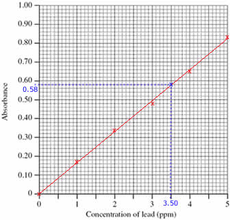
- Plot the calibration curve using the concentrations and absorbances of the standard solutions (shown as red x's on the graph)
- Draw a line of best fit through the plotted points (shown as a red line on the graph)
Step 2: Use the calibration curve to find the concentration of lead in the sample:
- Mark the position of the 0.58 absorbance of the sample being investigated (shown on the graph as a blue x)
(Draw a horizontal line, parallel to the x axis, from absorbance 0.58 until it meets the line drawn on the graph. Shown on the graph as a dotted blue line.)
- Read off the concentration of lead in the sample from the graph, 3.50 ppm
(From the blue x on the line in the graph, draw a line vertically down to meet the x axis. Shown on the graph as a dotted blue line.)
The concentration of lead in the sample was 3.50 ppm.
(Check that your answer is sensible. The absorbance of the sample lies between the absorbance for standards 3 and 4, therefore the concentration of lead in the sample must be between 3.00 and 4.00 ppm)
Example : Diluted Sample
Samples are often diluted before being analysed.
When this occurs, you will need to take this into account when you calculate the concentration of the original sample.
A student prepared standard lead solutions for comparison and the aborbance of each solution was measured.
A road-side soil sample was also prepared.
10 mL of this prepared soil sample was placed in a 100 mL volumetric flask and enough water was added to make it up to the mark.
The absorbance of this diluted soil sample was recorded.
The results are shown in the table below.
| Sample | Concentration (ppm) | Absorbance |
|---|
| Blank |
0.00 |
0.00 |
| Standard 1 |
1.00 |
0.17 |
| Standard 2 |
2.00 |
0.34 |
| Standard 3 |
3.00 |
0.48 |
| Standard 4 |
4.00 |
0.65 |
| Standard 5 |
5.00 |
0.83 |
| Sample |
? |
0.26 |
What was the concentration of lead in the original (undiluted) soil sample?
Step 1: Draw the calibration curve
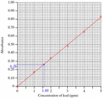
- Plot the calibration curve using the concentrations and absorbances of the standard solutions (shown as red x's on the graph)
- Draw a line of best fit through the plotted points (shown as a red line on the graph)
Step 2: Use the calibration curve to determine the concentration of lead in the diluted sample
- Mark the position of the 0.26 absorbance of the sample being investigated (shown on the graph as a blue x)
(Draw a horizontal line, parallel to the x axis, from absorbance 0.26 until it meets the line drawn on the graph. Shown on the graph as a dotted blue line.)
- Read off the concentration of lead in the diluted sample from the graph, 1.60 ppm
(From the blue x on the line in the graph, draw a line vertically down to meet the x axis. Shown on the graph as a dotted blue line.)
- Concentration of lead in the diluted sample was 1.60 ppm
(Check that your answer is sensible. The absorbance of the sample lies between the absorbance for standards 1 and 2, therefore the concentration of lead in the sample must be between 1.00 and 2.00 ppm)
Step 3: Calculate the concentration of lead in the original, undiluted sample.
Using logic:
- Concentration of lead in the diluted sample was 1.60 ppm (see above calculations)
Since 1 ppm = 1 mg L-1
1.60 ppm = 1.60 mg L-1
Concentration of lead in diluted sample = 1.60 mg L-1
- Therefore the concentration of lead in the 100 mL volumetric flask used for the dilution was 1.60 ppm or 1.60 mg L-1
- The mass of lead in the 100 mL volumetric flask = concentration (mg/L) x volume (L)
concentration = 1.60 mg/L
volume = 100 mL = 100/1000 L = 0.100 L
mass of lead in 100 mL volumetric flask = 1.60 mg/L x 0.100 L = 0.16 mg
- All the lead in the volumetric flask came from the 10 mL sample of the original solution.
Therefore the 10 mL undiluted sample contained 0.16 mg of lead.
- Concentration of lead in the 10 mL undiluted sample = mass (mg) ÷ volume (L)
mass (mg) = 0.16 mg
volume (L) = 10 mL = 10/1000 L = 0.010 L
concentration of lead in undiluted sample = 0.16 mg ÷ 0.010 L = 16 mg L-1
Since 1 mg L-1 = 1 ppm
16 mg L-1 = 16 ppm
Lead concentration in the sample of road-side soil was 16 ppm (or 16 mg L-1).
(Check that your answer is sensible. Since the original sample has been diluted, the concentration of the original undiluted sample must be greater than the concentration of the diluted sample used in the AAS experiment)
Using dilution equation (formula):
- c1V1 = c2V2
c1 = lead concentration in undiluted sample = ? ppm
V1 = volume of undiluted sample in litres = 10/1000 = 0.010 L
c2 = lead concentration in diluted sample = 1.60 ppm
V2 = volume of diluted sample in litres = 100/1000 = 0.100 L
- Substitute the values into the equation and solve:
c1 x 0.010 = 1.60 x 0.100
c1 x 0.010 = 0.16
c1 = 0.16 ÷ 0.010
c1 = 16 ppm
Lead concentration in the sample of road-side soil was 16 ppm (or 16 mg L-1).
(Check that your answer is sensible. Since the original sample has been diluted, the concentration of the original undiluted sample must be greater than the concentration of the diluted sample used in the AAS experiment)